Supplementary Research Results

Iwan Meier and Vefa Tarhan, "Corporate Investment Decision Practices and the Hurdle Rate Premium Puzzle"

This document contains a collection of tables and graphs that are not displayed in the paper. Some of the results are reported in the text. The additional tables and graphs are presented using the section headings from the paper. To distinguish the numbering from the one in the paper, we use the section and consecutive letters to identify these additional tables and figures, e.g. Table II.B.a for the first table in Section II.B, or Figure V.B.b for the second table in Section V.B.

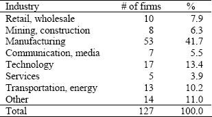
Table I.B.a: Number of firms by industry.

Table I.B.b: Breakdown of firms by size.

Size is measured by self-reported sales from the survey. The percentages in the last column correspond to Figure 2, Panel B.

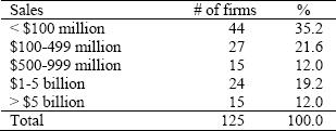
Table I.B.c: Firms with multiple business lines.

The table summarizes the # of responses to the question: “Does your firm have multiple product lines?”

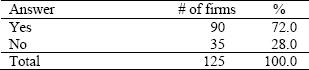
Table I.B.d: Company ownership.

The table summarizes the # of public and private firms in our sample.

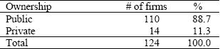
Table I.B.e: Equity stake of senior management.

The table summarizes the 107 quantitative answers to the question: “What is the approximate equity stake of senior management in the firm?” Five answers to this question were either <1%, <5%, or <8%. In these cases we take the exact values 1%, 5%, and 8%. Similarly, the two responses 50%+ and >1% are replaced by 50% and 1%. An additional 15 respondents checked the box “Don’t know.”

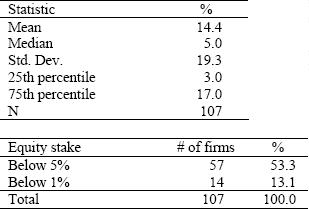
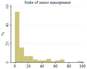
Figure I.B.a: Equity stake of senior management.

The histogram shows the distribution of the equity stake of senior management. Table I.B.e reports the corresponding summary statistics. The number of quantitative responses from the survey is 107. Five answers to this question were either <1%, <5%, or <8%. In these cases we take the exact values 1%, 5%, and 8%. Similarly, the two responses 50%+ and >1% are replaced by 50% and 1%.

II. Self-reported Hurdle Rates

II.A Summary Statistics on Hurdle Rates

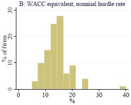
Table II.A.a: Summary statistics for unadjusted and WACC equivalent, self-reported hurdle rates.

The table shows summary statistics of the self-reported hurdle rates that are taken directly from the survey without any adjustments; the WACC equivalent, self-reported hurdle rates; and the WACC equivalent hurdle rates for firms that always use the company-wide hurdle rate when evaluating projects. The hurdle rates represent the nominal rate that the company has used for a typical project during the previous two years. In the second column, self-reported hurdle rates that represent the cost of levered or unlevered equity are converted to their WACC equivalents. This conversion procedure is explained in Section II.C of the paper. These numbers are the ones reported in Table I and are reproduced to facilitate comparisons. The last column reports the summary statistics for firms that, according to a separate survey question, use always the company-wide hurdle rate.

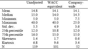
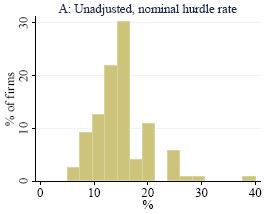
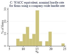
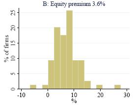
Figure II.A.a: Unadjusted and WACC equivalent, self-reported hurdle rates.

The histogram plots the unadjusted, self-reported hurdle rates (Panel A) and the WACC equivalent, self-reported hurdle rates (Panel B) that the firms have used for a typical project during the last two years (in nominal terms). Panel C reports the WACC equivalent, self-reported hurdle rates for the 52 firms that always use the company-wide hurdle rate when evaluating projects. The columns of Table II.A.a report the corresponding summary statistics.

II.B What Do Hurdle Rates Represent?

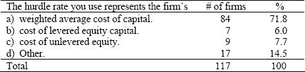
Table II.B.a: What the hurdle rate represents.

The table shows what the survey participants claim the hurdle rates they provide in the survey represent. The percentages in the last column correspond to Figure 3 in the paper.

II.C Converting Non-WACC Self-reported Hurdle Rates to WACC-based Self-reported Hurdle Rates

III. WACC Computations for the Survey Firms

III.A Computing Cost of Levered Equity Using CRSP and Compustat Data

Table III.A.a: Summary statistics for the typical project life.

The table summarizes the 124 responses to the question “What is the typical life of a project that your firm considers?” Four respondents answered 10+, 5+, or 2+. In these cases we use a multiplier of 1.5 to calculate the upper limit. For example, we assign a range of 10 to 10 × 1.5 = 15 and hence an average project life of 12.5 years. Similarly, we substitute the answer “majority less than 1 year, none exceed 2 years” with a range from 1/1.5 = 0.67 to 2 and set the average to 1.33. The answer “R+D 5-10 years, [investments into] capital 3-5 years” is replaced by a range of 3-10 and a corresponding average life of 6.5, and “0-1, some to 10 years” with 0-10 and an average life of 1 year.

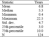
Table III.A.b: Pairwise correlations between different beta estimates.

The correlation matrix shows the pairwise correlation coefficients for seven beta estimates and, in the last column, when for each individual firm the maximum of all beta estimates is taken. The details of the beta estimations are described in the caption of Table 2 and in Appendix A.2 of the paper. The number of observations varies from 92 to 94, depending on whether the estimates use monthly, weekly (92), daily data (93), or an industry average (94). Since adjusted beta is just a scaled version of the beta from 5-year monthly data, the correlation coefficients for the two measures are the same.

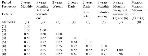
Table III.A.c: Spearman rank order correlations between different beta estimates.

Same as Table III.A.b reporting the non-parametric Spearman rank order correlations instead of the linear correlation coefficient. The details of the beta estimations are described in the caption of Table 2 and in Appendix A.2 of the paper. The number of observations varies from 92 to 94, depending on whether the estimates use monthly, weekly (92), daily data (93), or an industry average (94).

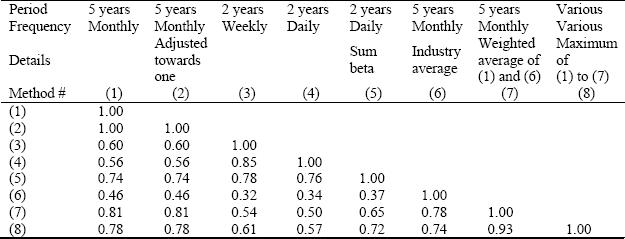
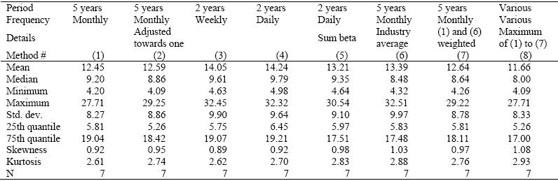
Table III.A.d: Summary statistics for cost of levered equity; equity premium of 6.6%.

The table shows summary statistics for the cost of equity for the sample firms where we can match with Compustat data. In calculating cost of equity from the Capital Asset Pricing Model (CAPM) we compare the results for the seven different methods to estimate beta coefficients. The parameters for the CAPM are 4.3% for the risk-free rate (the rate for 10-year Treasury bonds at the time of the survey at the end of October 2003) and a historical equity premium of 6.6% (the average excess return of the large stocks over long-term bonds from January 1926 to December 2003). The specific regressions we run are detailed in the caption of Table 2 and explained in Appendix A.2. The last column, method (8) provides the results when we use for each individual firm the maximum beta from methods (1) to (7).

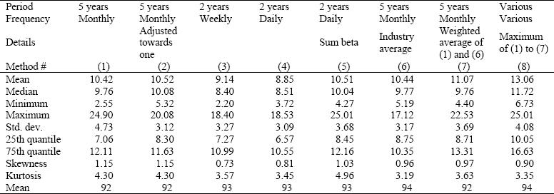
Table III.A.e: Summary statistics for cost of levered equity; equity premium of 3.6%.

The table shows summary statistics for the cost of equity for the sample firms where we can match with Compustat data. In calculating cost of equity from the Capital Asset Pricing Model (CAPM) we compare the results for the seven different methods to estimate beta coefficients. The parameters for the CAPM are 4.3% for the risk-free rate (the rate for 10-year Treasury bonds at the time of the survey at the end of October 2003) and the median of the CFO forecasts for the equity premium on December 2003 as documented in Graham and Harvey (2006). The specific regressions we run are detailed in the caption of Table 2 and explained in Appendix A.2. The last column, method (8) provides the results when we use for each individual firm the maximum beta from methods (1) to (7).

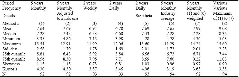
Figure III.A.a: Typical project life.

The histogram summarizes the 124 answers to the question: “What is the typical life of a project that your firm considers?” For firms providing a range rather than one number (38.7% of the respondents) we use the average. Table III.A.a tabulates the summary statistics.

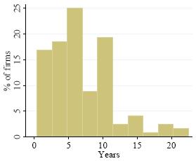
Figure III.A.b: Range for the typical project life.

The histogram shows the distribution of the ranges. For all observations (including the 76 surveys with range zero) the mean is 1.9 years with a standard deviation of 4.0 years. The value for the 75th percentile is 2 years and for the 90th percentile it is 5 years. There was one firm with a range of 1-30 years followed by the second largest ranges of 15-30 years and 5-20 years.

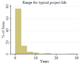
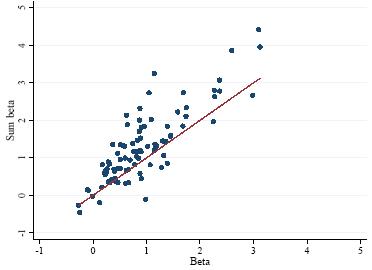
Figure III.A.c: Beta vs. sum beta using two year of daily data.

The beta estimates in this graph are based on regressions using two years of daily data from January 2002 to December 2003. The beta on the horizontal axis, beta, results from a regression of dividend-adjusted stock returns, , on the S&P 500 index returns,: . The sum beta on the vertical axis adds the coefficients of a similar regression on the concurrent and four lagged values of the S&P 500:, then the sum beta equals. These beta estimations correspond to Models (4) and (5) as described in the Appendix A.2 in the paper. The solid line plots the 45° line. The graph shows the results for the 93 publicly traded companies with matching daily returns from CRSP.

III.B After-tax Cost of Debt, Debt/Equity Weights and the WACC Computations

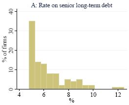
Table III.B.a: Summary statistics for rates on senior, long-term debt.

We report summary statistics for the 88 self-reported rates on senior long-term debt together with the 12 firms for which we infer the rate using the Z-score. For Z-scores of three and above we use the 10-year Treasury rate of 4.3% in October 2003 plus 1%; for Z-scores between 1.81 and 3, we assign a rate of T-bond rate plus 2.5%; and for firms with a Z-score below 1.81 the long-term bond rate is set to T-bond rate plus 4%. Self-reported rates below the 10-year Treasury rate of 4.3% are corrected to 4.8%. The 16 firms that had no debt are not included in the second column.

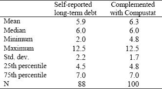
Table III.B.b: Summary statistics on tax rates.

Tax rates are computed as total income taxes divided by income before taxes. In case one of the input variables is negative we assign a tax rate of zero. Tax rates are also capped at 34%.

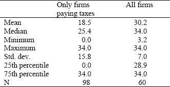
Table III.B.c: Changes in capital structure over the next three years.

We ask survey participants whether their company, compared with the current capital structure, has the intention to change its capital structure over the next three years.

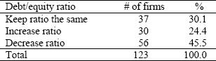
Table III.B.d: Summary statistics for weighted average cost of capital (WACC); equity premium of 6.6%.

The table shows summary statistics for the weighted average cost of capital (WACC) for the sample firms where we can match with Compustat data. In calculating cost of equity from the Capital Asset Pricing Model (CAPM) we compare the results for the seven different methods to estimate beta coefficients. The parameters for the CAPM are 4.3% for the risk-free rate (the rate for 10-year Treasury bonds at the time of the survey at the end of October 2003) and a historical equity premium of 6.6% (the average excess return of the large stocks over long-term bonds from January 1926 to December 2003). The specific regressions we run are detailed in the caption of Table 2 and explained in Appendix A.2. The last column, method (8) provides the results when we use for each individual firm the maximum beta from methods (1) to (7).

Table III.B.e: Summary statistics for weighted average cost of capital (WACC); equity premium of 3.6%.

The table shows summary statistics for the weighted average cost of capital (WACC) for the sample firms where we can match with Compustat data. In calculating cost of equity from the Capital Asset Pricing Model (CAPM) we compare the results for the seven different methods to estimate beta coefficients. The parameters for the CAPM are 4.3% for the risk-free rate (the rate for 10-year Treasury bonds at the time of the survey at the end of October 2003) and the median of the CFO forecasts for the equity premium on December 2003 as documented in Graham and Harvey (2006). The specific regressions we run are detailed in the caption of Table 2 and explained in Appendix A.2. The last column, method (8) provides the results when we use for each individual firm the maximum beta from methods (1) to (7).

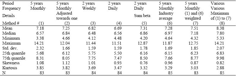
Table III.B.f: Summary statistics for weighted average cost of capital (WACC), only for firms using WACC as their hurdle rate; equity premium of 6.6%.

The table shows the same summary statistics for the weighted average cost of capital (WACC) under the 6.6% equity premium scenario as as Table III.B.d. However, only those firms are included which claim that their hurdle rate represents WACC.

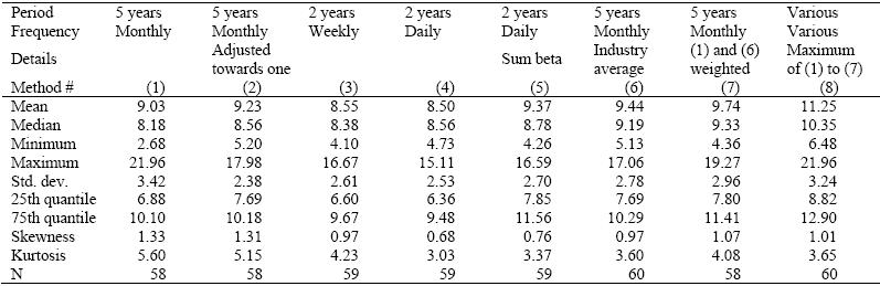
Table III.B.g: Summary statistics for weighted average cost of capital (WACC), only for firms using WACC as their hurdle rate; equity premium of 3.6%.

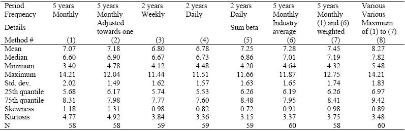
Figure III.B.a: Approximations for the rate on senior long-term debt and tax rates.

The histogram in Panel A shows the distribution of returns on long-term debt. The rates are imputed from self-reported rates, complemented with Compustat data. We perform a few adjustments that are explained in Section III.B in the paper. Panel B summarizes the tax rates that we infer from the quotient tax payments/income before taxes in 2003. If any of the input variables is negative we set the tax rate equal to zero. The tax rates are capped at 34%.

IV. Documenting the Existence of the Hurdle Rate Premium Puzzle

Table IV.a: Unadjusted, self-reported hurdle rate minus cost of equity; equity premium 6.6%

This table provides summary statistics for the difference between the unadjusted hurdle rate, that is directly taken form the survey, and the cost of equity computed from CRSP and Compustat. The seven beta estimation methods are detailed in the caption of Table 2 and explained in Appendix A.2. The last column, method (8), provides the results when we use for each individual firm the maximum beta from methods (1) to (7). The equity premium assumption is 6.6%.

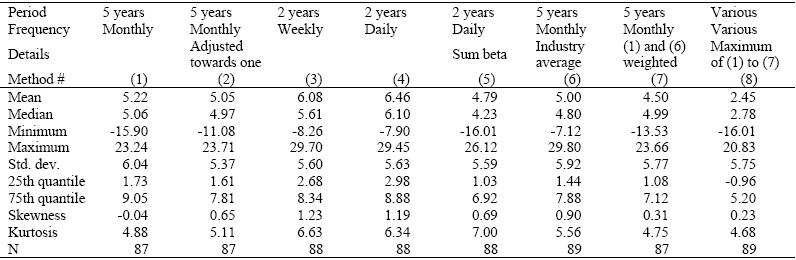
Table IV.b Unadjusted, self-reported hurdle rate minus cost of equity; equity premium 3.6%

This table provides summary statistics for the difference between the unadjusted hurdle rate, that is directly taken form the survey, and the cost of equity computed from CRSP and Compustat. The seven beta estimation methods are detailed in the caption of Table 2 and explained in Appendix A.2. The last column, method (8), provides the results when we use for each individual firm the maximum beta from methods (1) to (7). The equity premium assumption is 3.6%.

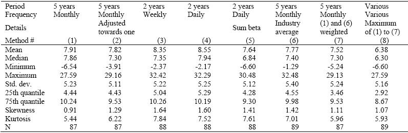
Table IV.c: Summary statistics for hurdle premium = hurdle rate – weighted cost of capital (WACC); equity premium 6.6%.

Same as Table 3 in the paper for all eight methods. The equity premium is set to the historical equity premium of 6.6% (the average excess return of the large stocks over long-term bonds from January 1926 to December 2003).

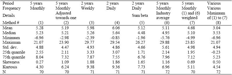
Table IV.d: Summary statistics for hurdle premium = hurdle rate – weighted cost of capital (WACC); equity premium 3.6%.

Same as Table 3 in the paper for all eight methods. The equity premium is set to 3.6%, corresponding to the median forecast of the CFOs responding in December 2003 to the Duke/CFO Magazine as reported in Graham and Harvey (2006).

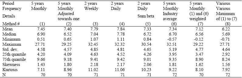
Table IV.e: Summary statistics for premium above cost of levered equity = hurdle rate – cost of levered equity; equity premium 6.6%.

We define the premium above cost of levered equity as the difference between the self-reported hurdle rate and the cost of levered equity reported in Table III.A.d. The table reports summary statistics for the cross-section of firms that revealed their identity and are publicly traded such that we can match the corresponding returns on equity from CRSP. We estimate cost of equity using the Capital Asset Pricing Model (CAPM) to estimate the cost of equity. For details on these beta coefficients see the caption of Table 2 and the Appendix A.2 of the paper. The parameters used for the CAPM are 4.3% for the risk-free rate (the rate for 10-year Treasury bonds at the time of the survey at the end of October 2003) and a historical equity premium of 6.6% (the average excess return of the large stocks over long-term bonds from January 1926 to December 2003). The table shows the results for different approaches to estimate the beta coefficient. The last column tabulates the statistics when for each individual firm the maximum beta estimates from the methods (1) to (7) is taken.

Table IV.f: Summary statistics for premium above cost of levered equity = hurdle rate – cost of levered equity; equity premium 3.6%.

We define the premium above cost of levered equity as the difference between the self-reported hurdle rate and the cost of levered equity reported in Table III.A.e. The table reports summary statistics for the cross-section of firms that revealed their identity and are publicly traded such that we can match the corresponding returns on equity from CRSP. We estimate cost of equity using the Capital Asset Pricing Model (CAPM) to estimate the cost of equity. For details on these beta coefficients see the caption of Table 2 and the Appendix A.2 of the paper. The parameters used for the CAPM are 4.3% for the risk-free rate (the rate for 10-year Treasury bonds at the time of the survey at the end of October 2003) and the median CFO forecast for the equity premium of 3.6% (in December 2003), as reported by Graham and Harvey (2006). The table shows the results for different approaches to estimate the beta coefficient. The last column tabulates the statistics when for each individual firm the maximum beta estimates from the methods (1) to (7) is taken.

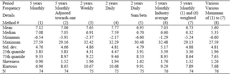
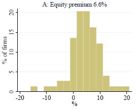
Figure IV.a: Hurdle premium above cost of levered equity.

The hurdle premium is defined as the difference between the WACC based, self-reported hurdle rate and the cost of levered equity we compute from CRSP and Compustat. We use the Capital Asset Pricing Model (CAPM) to infer the cost of equity. The parameters we use are 4.3% for the risk-free rate (10-year Treasury bond rate in October 2003) and two equity premium scenarios: 6.6% and 3.6%. Beta coefficients are inferred from a regression of monthly returns for the firm on returns on the S&P 500 over the past five years.

V. Investigation of the Hurdle Rate Premium Puzzle

V.A. Determinants of the Hurdle Rate Premium Puzzle: Bivariate Regressions

Table V.A.a: Bivariate regressions of the self-reported hurdle rate on selected financial variables.

Similar to Table 4 in the paper, we report the bivariate regression results for self-reported hurdle rates as the dependent variable y.

The table shows the set of explanatory variables in the first column, the estimated coefficients a and b along with the t-statistics in parenthesis below, and the R-squares. The table reproduces the regression results for the 6.6% equity premium scenario from Table 4 and additionally reports the same regressions for the 3.6% scenario. For the details on the explanatory variables, the reader is referred to Table 4 in the paper. Significantly different from zero at the 1% level ***; at the 5% level **; at the 10% level *.

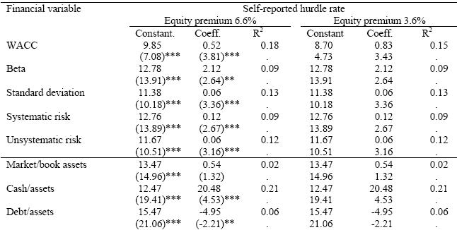
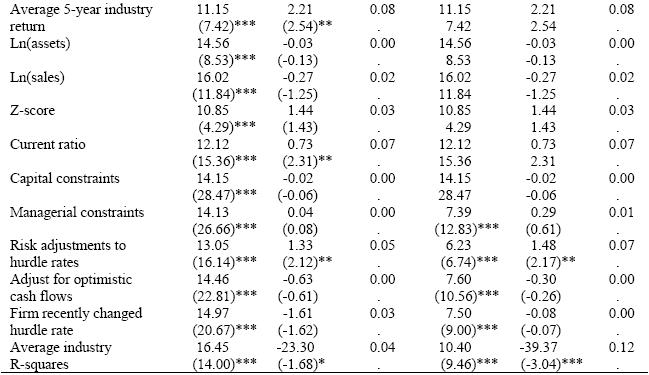
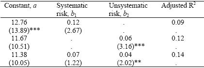
Table V.A.b: Relative importance of systematic risk versus unsystematic risk in explaining the self-reported hurdle rates and the hurdle premium.

The table summarizes the results from regressions of the hurdle rate (Panel A) and the hurdle premium (Panel B), defined as the difference between hurdle rate and computed WACC, against systematic risk, unsystematic risk, and both. In case of the hurdle premium, two scenarios for the equity premium are considered: 6.6% and 3.6%. For each dependent variable we tabulate the results from three regressions. The cells contain the estimated coefficients with the t-statistics below, and the adjusted R-squares of the regressions. In these tables the explanatory variables are arranged in the columns.

Panel A: Self-reported hurdle rate.

Panel B: Hurdle premium.

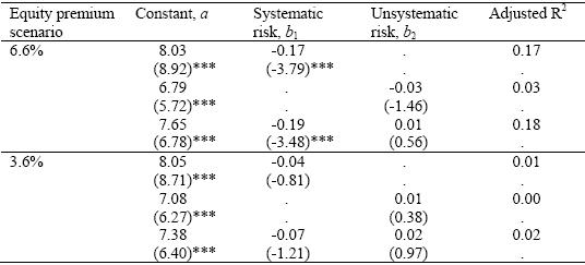
Table V.A.c Hurdle premium for the 7 firms that use cost of levered equity to discount, equity premium 6.6%.

Table V.A.d Hurdle premium for the 7 firms that use cost of levered equity to discount, equity premium 3.6%.

V.B Determinants of the Hurdle Rate Premium Puzzle: Multivariate Regressions

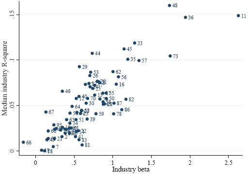
Figure V.B.a Relationship between median industry R-beta and R-squares.

Scatter plot of the median R-square of the beta estimations for all firms within the same two-digit SIC code using 5 years of monthly data against the median beta coefficient within the same two-digit SIC category. The graph plots only the industries that are represented by our sample firms. The markers are labeled with their corresponding two-digit SIC code. The legend below for the SIC codes is sorted by median industry betas.

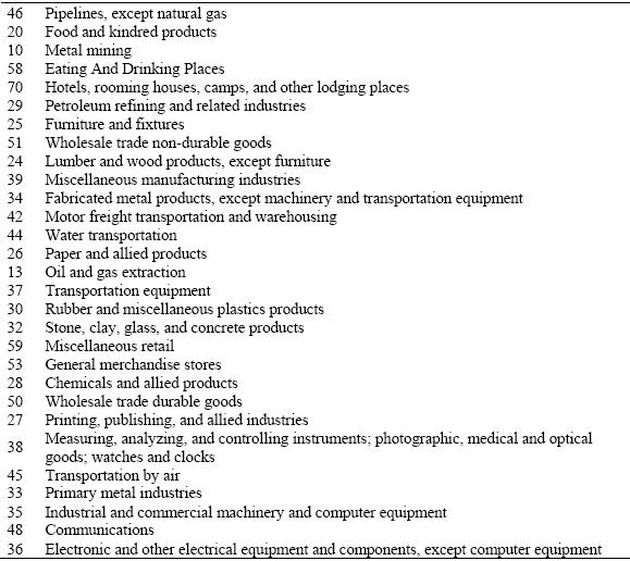
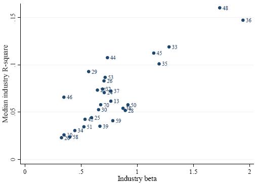
Figure V.B.b Relationship between median industry R-beta and R-squares.

Same as in 5.1.A, however including all two-digit SIC codes with at least 20 firms with monthly data in CRSP from January 1998 to December 2003.

V.C Other Possible Explanations of the Hurdle Rate Premium Puzzle

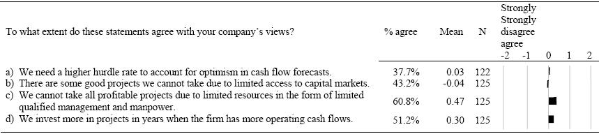
Table V.C.a: Potential explanations for the hurdle premium: Survey data.

The table shows the fraction of the responding firms that strongly agree or agree (scores of 2 and 1 on a scale from -2 to 2), the mean, and the number of respondents. The bars illustrate the means.

VI. Cashflow Related Practices and Interactions between Cashflows and Hurdle Rates

VI.A Calculation of Cashflows, Sunk Costs, and Cannibalization of Existing Product Sales

Table VI.A.a: Foreign investments.

Only firms with foreign investments answered this question (57 respondents to the first question and 52 to the second question).

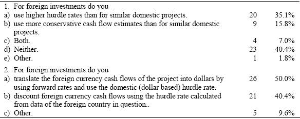
Figure VI.A.a: Calculation of cash flows.

The bar chart summarizes how firms calculate cash flows in evaluation projects. EBIAT is earnings before interest and after taxes, D denotes depreciation, CAPX capital expenditures, and dWK the net change in working capital. The bar chart illustrates the results of Table 7 in the paper.

VI.B. Interactions between Cashflows and Hurdle Rates

VII. Self-Reported Hurdle Rates Revisited

VII.A Frequency of Hurdle Rate Changes

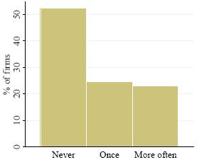
Table VII.A.a: Hurdle rate changes over the past three years.

The table reports the number of firms and the fraction out of the 122 respondents to this question.

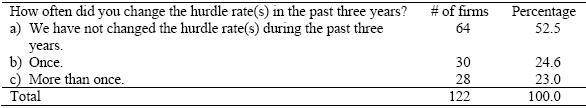
Figure VII.A.a: Hurdle rate changes over the past three years.

The graph illustrates the answers to the question; “How often did you change the hurdle rate(s) in the past three years?” The questionnaire offers three possible choices: (i) We have not changed the hurdle rate(s) during the past three years (labeled in the graph as “Never”); (ii) once; and (iii) more than once. The corresponding numbers are displayed in Table VII.A.a.

VII.B Multi-Segment Firms and Use of Firm-Wide versus Divisional Hurdle Rates

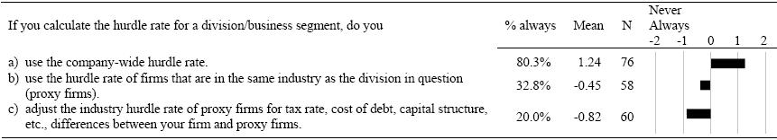
Table VII.B.a: Divisional hurdle rates.

The table reports how firms with multiple divisions or business segments adjust their hurdle rates. In a separate question, a total of 79 firms answer that they actually have multiple divisions. The table shows the fraction of the responding firms that would always use the method in question, the mean of all answers on the scale from -2 (never) to 2 (always), and the number of respondents. The bars plot the means. As a percentage of the 76 firms answering to a), the fractions of firms answering 1 or 2 in b) and c) are 25.0% and 15.8%.

VII.C Strategic Projects

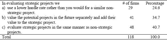
Table VII.C.a: Strategic projects.

The table show the results on how firms evaluate strategic projects which are defined in the questionnaire as “projects where accepting a given project today may enable the firm to make additional future investments.”

VIII. Capital Budgeting Methods

Table VIII.a: Capital budgeting methods.

The table tabulates the number of firms illustrated in Figure 5 of the paper. For the eleven respondents that do not provide a ranking, a rank of one is assigned to all methods checked. Therefore, the total of first choices (149) exceeds the number of 126 respondents to this question. The number of second choices (85) is substantially lower as some firms mainly rely on a single technique.

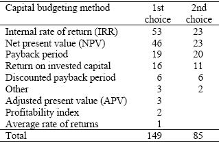
Table VIII.b: Use of DCF, NPV/IRR as first choice

88.1% of the 126 respondents use discounted cash flow techniques (DCF) as their first or second choice. DCF includes net present value (NPV), adjusted present value (APV), internal rate of return (IRR), and profitability index (PI). 85.8% use NPV or IRR as one of their two most important capital budgeting techniques.

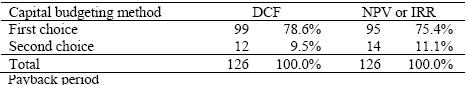
Figure VIII.a: Payback period.

The histograms illustrate the lower and upper bounds that firms use as the required payback or discounted payback period. There are 79 respondents to this question. 37 CFOs do explicitly not use the (discounted) payback method for any project.

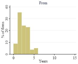
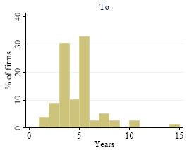
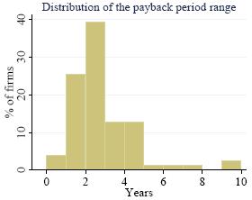
Figure VIII.b: Bandwidth of payback periods.

Distribution of the difference between the maximum and minimum for the required (discounted) payback period. The mean of the bandwidth used for payback is 2.4 years with a standard deviation of 1.7. As the distribution is skewed to the right the median is slightly lower at 2.0 years. The number of respondents is 79, the same as in Figure VIII.a.

IX. Conclusions

Appendices

A.1 Age, Experience, and Education of the Respondents

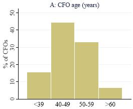
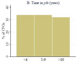
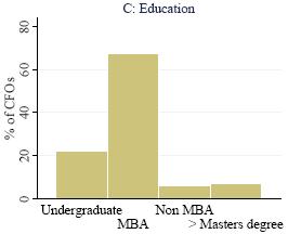
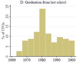
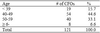
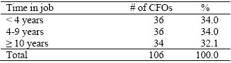
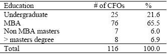
Table A.1.A: CFO characteristics.

Information about the CFOs completing the form. The three characteristics are age, time in job, and education.

A.2 Beta Coefficient Estimation Procedures

Figure A.2.A: CFO Profiles.

The four panels illustrate the characteristics of the CFOs completing the form: Age, time in current job, education, and the year when the person graduated the last time.